Every university goes through an annual budgeting cycle. There are about as many budget processes as there are universities but they all have one thing in common: the need to take account of changes in enrolment, governmental support, and other external factors. This is not easy because each potential factor affects various parts of the institution in different ways, each of which may have different implications for budget making. Previous blogs have described how the Pilbara model can inform program changes, decisions about course delivery methods, tuition-setting, and many other decisions that have implications for budgeting. In this one we focus more broadly on analysing the external factors, with the objective of improving the budget process.
The basic idea is that because Pilbara provides a detailed description of the university’s teaching, research, and overhead operations, the model’s predictive version can be used to adjust last year’s spending to what will be required next year in light of changed external conditions. Considering enrolments, for example, one can use the predictive model to determine what changes in academic staff will be required to maintain current class sizes, teacher profiles, and research efforts. These adjustments are shown on a department-by department basis rather than as aggregates for schools or faculties. The model also traces the adjustments’ probable effects on overhead. Thus, academic decision-makers will be able to spend their time negotiating substantive issues like service levels and efficiency rather than trying to guess the consequences of predicted enrolment and workforce changes.
Scenario Planning
The ability to adjust for changed external conditions opens up yet another exciting possibility: Scenario Planning. A ‘planning scenario’ combines a set of predicted events with an assumed set of university responses. As in the real world, the events can represent complex combinations of external factors – e.g., enrolment changes, reductions in Government student funding, a dramatic shift in the global economy, or even a structural change like the’ half-cohort’ expected to hit Queensland universities in 2020 as a result of adding a Prep Year to the state’s primary schooling.
The university’s responses can be as complex as required to deal with the projected changes. Multiple actions of the kind discussed in our previous blogs can be included in the scenario. Use of the Pilbara predictive model allows what-if analysis to be performed in an extremely flexible yet rigorous way. The analyses can answer questions like, “Do we have enough students to break even?”, “How should we target different types of student so as to maximize our margins?” and “How do we set the price for fee paying students to ensure we aren’t making a loss?” Such questions are becoming more and more important as universities’ financial and competitive environments become more challenging.
The following visual provides two scenarios – a baseline scenario (grey) and the scenario containing two one-off events (capping of the Government’s CGS grant in 2018 and a drop in CGS enrolments in 2020 due to the 1/2 cohort reaching university age)[1].
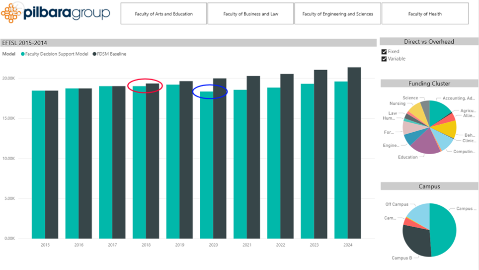
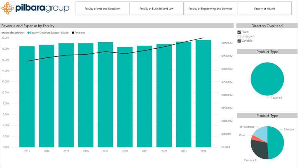
These simple events could be modelled in Excel – after all, they just show estimated EFTSL numbers based on a pair of straightforward assumptions. Even adding in the revenue adjustments based on the two events isn’t taxing: again quite simple to do in Excel.
The expense side is another story, however. Excel modelling of the changes to expenses, based on changes to the required teaching load, workload profiles and other variables would be almost impossible to do in a repeatable manner.
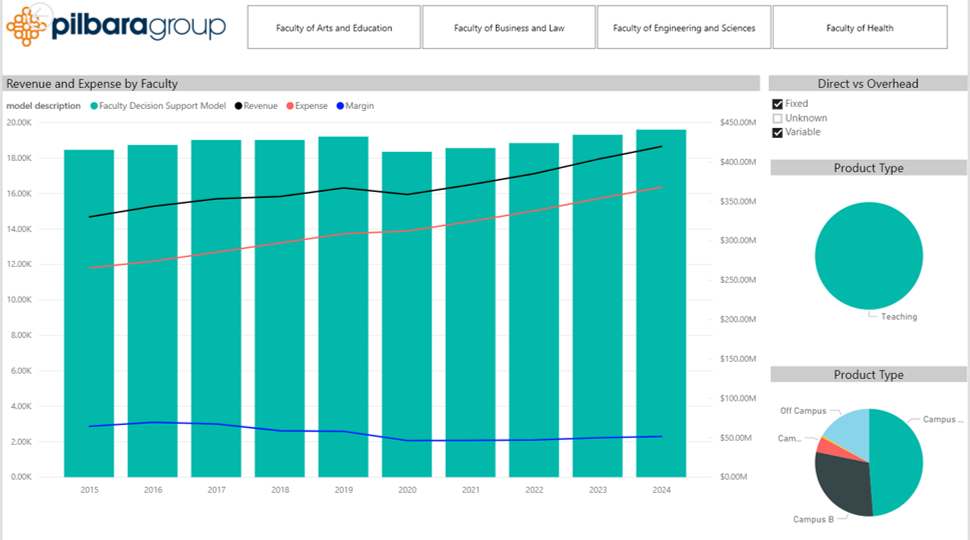
As can be seen here, the operating margin reduces in 2018 due to the capping of the CGS rates, and then before it gets a chance to recover, it is hit again, this time from the impact of the ½ cohort in 2020. The impact of this lasts for a minimum of 3 years as those students work through their degree.
From here, the university is then able to model new scenarios using this as the new baseline – what if they increase their market through online delivery, or additional Post Grad courses, or international students? What mix of these would be needed to offset the drop in margin and maintain a financially sustainable institution over the next 5-10 years?
The effort to calculate the changes to expenditure university-wide solely based on the 7% drop would be intensive, but to then run multiple scenarios, for example a 6% drop, an 8% drop, a change in the casual (sessional) / permanent workforce profile, a reduction in department (internal) research, a increase in online student, or a decrease in international students would be prohibitive in terms of effort without a model to support the ability to run these types of scenarios within minutes.
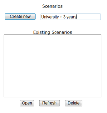
Any number of scenarios can be configured and compared, including ones that may seem unlikely but would have powerful consequences if they occur. Once these scenarios are developed and the model calculated, results can be presented in Microsoft Power BI or Excel, or using the online reporting tool provided with ACE, and direct comparisons between scenarios and previous performance figures can easily be seen. There is no need to manage scenarios in Excel, however. The Pilbara model provides a convenient way to create, store and manage whatever scenarios the user wishes to analyse.
Another example of how universities can use multiple scenarios to help with budgeting was discussed in the Blog Post “It’s a No-Brainer! Increasing Student Retention Makes Higher Ed More Money…Or Does it?”
The Pilbara historical model also can help improve student retention and degree attainment by helping to diagnose problem areas and identify places where the interventions discussed in that blog post may prove effective. The best place to start is with so-called ‘WFD’ (withdrawal, fail, D-grade) records, which can be included in the model if the institution makes the data available. These data enable identification of courses where students tend to have difficulty. A number of important lines of analysis and intervention follow from this important capability.
Searching for patterns in the data is one such inquiry. Using the historical model, one can compare the teaching methods, class sizes, instructor types, and instructors’ time commitments for courses with high and low WFD rates. Then, virtual experiments using the predictive model can estimate the staffing and cost implications of emulating the low-WFD configurations on a large scale (one might cap class sizes, for example, or reduce the use of adjuncts). Projecting WFD improvements from the virtual experiments doesn’t control for subject matter or student characteristics, but the staffing and cost estimates are based on solid data. In the end, of course, one would need to change on-the-ground course configurations and observe the actual results. For example, newspaper accounts of an experiment at the University of Texas-Austin’s Chemistry Department suggests that such experiments have a good chance of success. Using the Pilbara model to make WFD data available for all course instances in every semester will eliminate the time-consuming step of tracking individual student transcripts back to potentially problematic courses.
The predictive model also can be used to evaluate the staffing implications and costs of interventions to reduce bottlenecks in students’ progression toward their degrees. The bottlenecks are identified by looking at courses where capacity constraints cause would-be enrolees to be turned away, constraints that can be mitigated by adding sections. Then the Pilbara model can be used test the addition of sections in the same course instance, or the addition of new instances, to satisfy the disappointed students.
There are a wide-range of different types of scenarios that can be run in both the Historical Model and the Predictive Model. The objective is to allow better-informed decisions relating to budget setting and future planning to be based on actual data and models. It’s important to note that this sets a starting point for budget discussions, rather than using last year’s budget. Future year budgets can be estimated in the Predictive Model based on forecasted demand for teaching and research and then negotiations and iterative changes can be applied to this base budget.
Download the full whitepaper here: www.pilbara.co/whitepaper
[1] A 7% reduction is used for illustrative purposes – it could be higher for some QLD universities